Mastering in Data Science

The following technical blogs are coming to be covered in Data Science, Machine Learning & Analysis , visualization track. Be an enterprise Data Scientist by following the Data Scientist fast track modules: STAY TUNED!!

A lap around MACHINE LEARNING
Supervised and unsupervised learning
Kernel based methods
Text mining techniques
Performance evaluation

Exploring CATEGORICAL DATA ANALYSIS
Types of categorical data
Generalized linear models
Contingency tables
Simple and multinomial logistic regression models

Evaluation of STOCHASTIC PROCESSES AND SIMULATION
Random Variables and Distributions
Monte Carlo Simulation
Discrete Event Simulation
Variance Reduction Techniques

Data OPTIMIZATION Techniques
Linear Programming
Integer Programming
Multi-criteria Optimization
Goal Programming
AHP (Analytic Hierarchy Process)
Data Envelopment Analysis (DEA)

ECONOMETRIC METHODS in Data Science
Time Series Analysis
GARCH Models
Fixed Effects Estimation
Random Effects Estimation

STATISTICS for DATA SCIENCE
Probability Theory
Statistical Inference
Sampling Theory
Hypothesis Testing
Regression Analysis

Real World Case Studies in Data Science

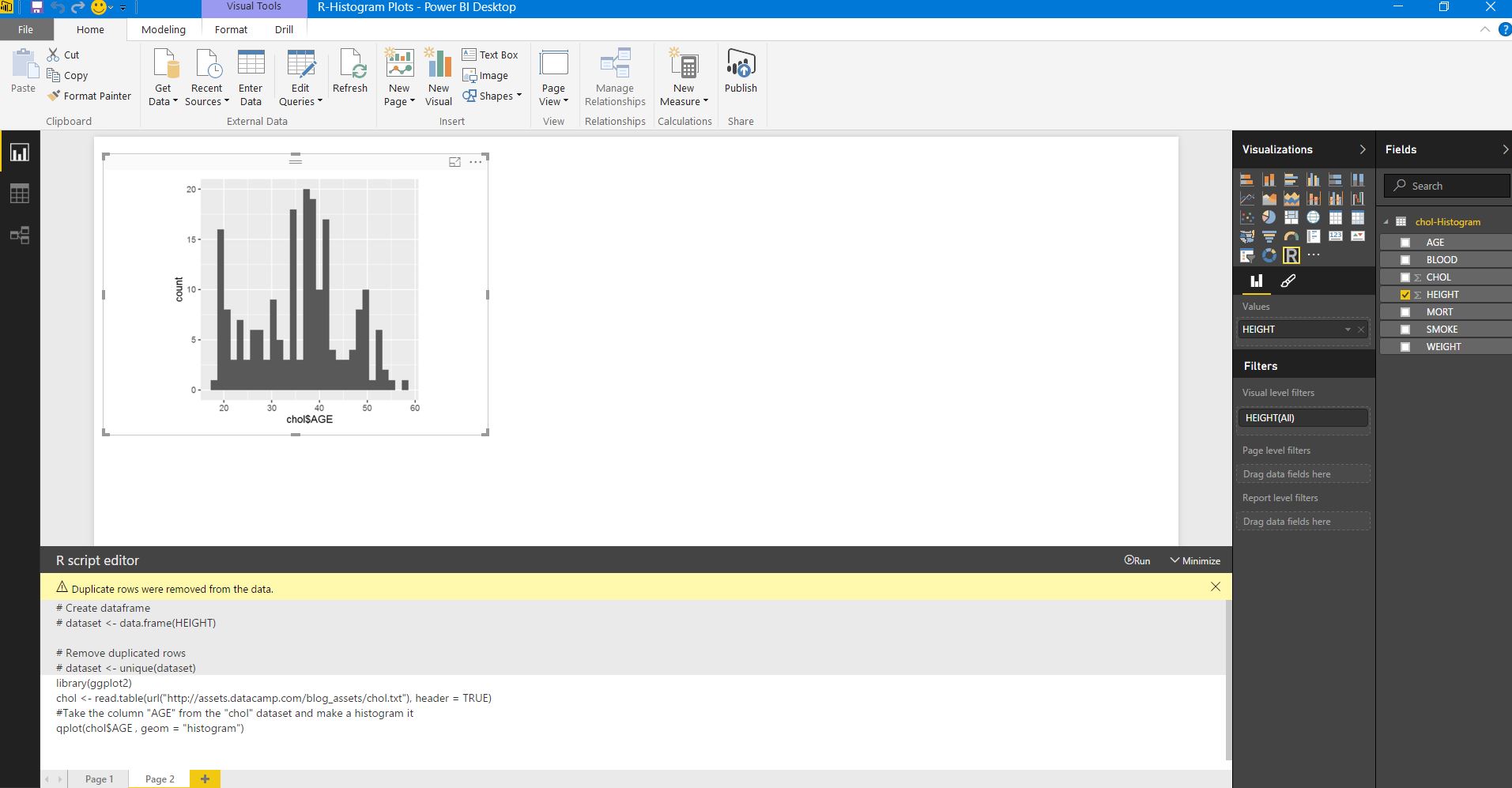
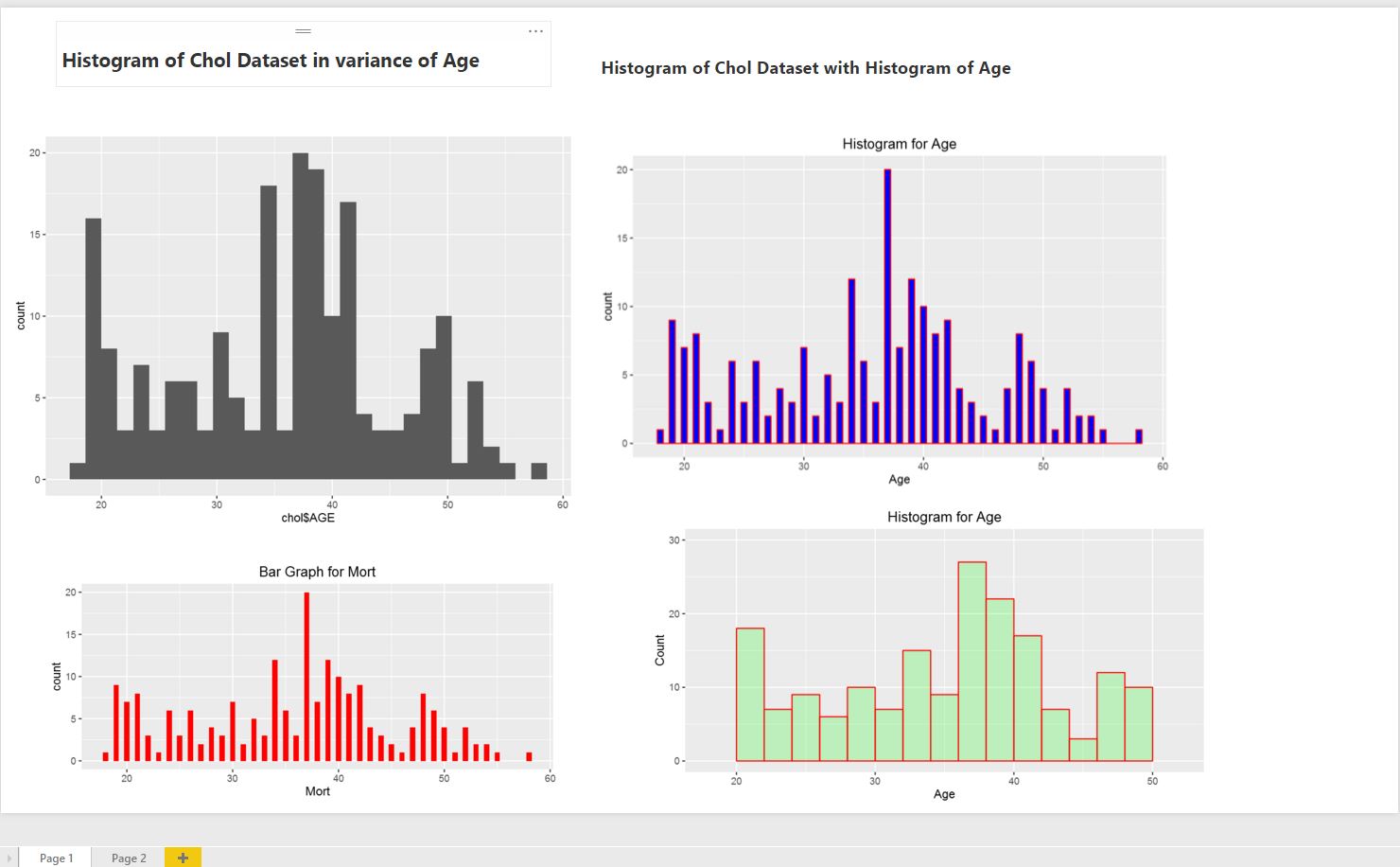
• Social Media Mining with R & Microsoft PowerBI

• Experimentation interactive R based visuals with Shiny apps

• What’s next with Julia

R with PowerBI – A step by step guide approach

A lot of interests are visible everywhere how to integrate R scripts with Microsoft PowerBI dashboards. Here goes a step by step guidance on this.

Lets assume, you have some couple of readymade R code available, for example , with ggplot2 library. Lets find the following scripts performing analytics using CHOL data.

1. Open R studio or R Package (CRAN) & install ggplot2 library first.

2. Paste the following R script & execute it.

install.packages(‘ggplot2’)
library(ggplot2)
chol <- read.table(url(“http://assets.datacamp.com/blog_assets/chol.txt&#8221;), header = TRUE)
#Take the column “AGE” from the “chol” dataset and make a histogram it
qplot(chol$AGE , geom = “histogram”)
ggplot(data-chol, aes(chol$AGE)) + geom_histogram()

you should be able to see the visuals output like this.

3. Next, execute the following pieces of R code to find out the binwidth argument using ‘qplot()‘ function.

qplot(chol$AGE,
geom = “histogram”,
binwidth = 0.5)

4. Lets take help of hist() function in R.

#Lets take help from hist() function
qplot(chol$AGE,
geom=”histogram”,
binwidth = 0.5,
main = “Histogram for Age”,
xlab = “Age”,
fill=I(“blue”))

5. Now, add I() function where nested  color.

#Add col argument, I() function where nested color.
qplot(chol$AGE,
geom=”histogram”,
binwidth = 0.5,
main = “Histogram for Age”,
xlab = “Age”,
fill=I(“blue”),
col=I(“red”))

6. Next, adjust ggplot2 little by the following code.

#Adjusting ggplot
ggplot(data=chol, aes(chol$AGE)) +
geom_histogram(breaks=seq(20, 50, by = 2),
col=”red”,
fill=”green”,
alpha = .2) +
labs(title=”Histogram for Age”) +
labs(x=”Age”, y=”Count”) +
xlim(c(18,52)) +
ylim(c(0,30))

7. Plot a bar graph with this following code.

#Plotting Bar Graph
qplot(chol$AGE,
geom=”bar”,
binwidth = 0.5,
main = “Bar Graph for Mort”,
xlab = “Mort”,
fill=I(“Red”))

8. Next, open PowerBI desktop tool. You can download it free from this link. Now, click on Get Data tab to start exploring & connect with R dataset. 

If you already have R installed in the same system building PowerBI visuals , you just need to paste the R scripts next in the code pen otherwise , you need to install R in the system where you are using the PowerBI desktop like this.

9. Next, you can also choose the ‘custom R visual’ in PowerBI desktop visualizations & provide the required R scripts to build visuals & finally click ‘Run’.

 

10. Build all the R function visuals by following the same steps & finally save the dashboard.

11.You can refresh an R script in Power BI Desktop. When you refresh an R script, Power BI Desktop runs the R script again in the Power BI Desktop environment.